PCA, IBS-based clustering, Fst and ADMIXTURE analysis
This sub-workflow carried out Admixture analysis, two different
Principal Component Analyses, and clustering based on Identity by State
distances and Fst . The first PCA is done with the function SmartPCA of
the
EIGENSOFT
software and performed with the argument run_smartpca. The second
one is done by using the function snpgdsPCA inside the R package
SNPRelate
and can be invoked with the argument run_gds_pca. Analysis with the
program Admixture are
carried out with the argument admixture. Both clustering are done
with Plink calculations of
Fst and IBS.
Description of the parameters:
genetic_structure: setting this to false will not run this
sub-workflowld_filt: an option to use LD-based filtering according to
parameters specified below, meaning to include or skip step 4ld_window_size: a window size in variant count or kilo bases (step
4)ld_step_size: number of variants to shift the window at the end of
each step (step 4)r2_value: squared correlation threshold; at each step, only pairs
of variants with r2 greater than the threshold are recognized (step 4)structure_remove_indi: the name of a file with listed samples that
will be removed in all of anylses in this sub-workflowsmartpca_param: the path to the file with additional parameters
for SmartPCA (step 6)pop_color_file: the path to the text file with specified color
codes for each population (steps 7, 9, 10 and 11)f_pop_marker: the path to the text file with specified marker
shapes for each population (steps 7 and 9)pca_yml: the path to the yml file containing the parameters to
plot interactive PCA results (steps 7 and 9)starting_k_value: starting number of clusters for Admixture
analysis (step 12)ending_k_value: maximal number of clusters for Admixture analysis
(step 12)cross_validation: the number of folds for cross-validation (step
13)termination_criteria: the lowest limit of the log-likelihood
change between iterations to stop the process of cross-validation
(step 13), option “-C” in program Admixtureplot_pop_order: the path to the text file with population IDs in
order they should be plotted on admixture graph (step 14)fst_based_nj_tree: an option to estimate NJ tree based on pairwise
Fst distances between each pair of populations (step 10)fst_nj_yml: the path to the yml file containing parameters of
plotting interactive NJ tree based on Fst (step 10)est_1_min_ibs_based_nj_tree: an option to estimate NJ tree based
on 1-ibs distance between each pair of samples in the dataset (step
11)ibs_nj_yml: the path to the yml file containing parameters of
plotting interactive NJ tree based on 1-ibs (step 11)Overview of the processed carried out in this sub-workflow:
Note: If your input files are already in Plink format, it will skip step 1) and step 2). Also, if the LD-based filtering is set to true, all the analyses will be carried out using LD-based pruned dataset.
Validation and test-run of the sub-workflow::
For workflow validation, we have downloaded publicly available samples (see map below) with whole genome sequences from NCBI database (Alberto et al., 2018; Grossen et al., 2020; Henkel et al., 2019). We included domestic goats (Capra hircus) represented by various breeds from Switzerland. In addition to them, we also included Alpine ibex (C. ibex) and Bezoar wild goat (C. aegagrus). Since we need an outgroup when performing some of the analyses, we also added Urial sheep (Ovis vignei). We will use variants from chromosome 28 and 29 of, all together, 85 animals.
 Geographic map of samples used for the testing and validation
purpose
Geographic map of samples used for the testing and validation
purpose
1. Required input data files
The input data should be in the VCF or PLINK binary format files.
All VCF files need to be splitted by the chromosomes and indexed with tabix. Please check test_files/test_input_vcf.csv or the example below, where, in our case, we inserted the link to the cloud stored data. The first information in each row of input file is chromosome id, next is path/to/the/file.vcf.gz and the last is path/to/the/file.vcf.gz.tbi. Please note that the chromosome id must not contain any punctuation marks.
chr28,https://data.cyverse.org/dav-anon/iplant/home/maulik88/28_filt_samples.vcf.gz,https://data.cyverse.org/dav-anon/iplant/home/maulik88/28_filt_samples.vcf.gz.tbi
chr29,https://data.cyverse.org/dav-anon/iplant/home/maulik88/29_filt_samples.vcf.gz,https://data.cyverse.org/dav-anon/iplant/home/maulik88/29_filt_samples.vcf.gz.tbi
In addition to the VCF input format, it is also necessary to prepare a sample map file of individuals and populations. Sample map has two tab-delimited columns: in the first column are individual IDs and in the second are population IDs as demonstrated on the example below. It is also important that the name of the file ends with “.map”.
SRR8437780ibex  AlpineIbex
SRR8437782ibex  AlpineIbex
SRR8437783ibex  AlpineIbex
SRR8437791ibex  AlpineIbex
SRR8437793ibex  AlpineIbex
SRR8437799ibex  AlpineIbex
SRR8437809ibex  AlpineIbex
SRR8437810ibex  AlpineIbex
SRR8437811ibex  AlpineIbex
SRX5250055_SRR8442974   Appenzell
SRX5250057_SRR8442972   Appenzell
SRX5250124_SRR8442905   Appenzell
SRX5250148_SRR8442881   Appenzell
SRX5250150_SRR8442879   Appenzell
SRX5250151_SRR8442878   Appenzell
SRX5250153_SRR8442876   Appenzell
SRX5250155_SRR8442874   Appenzell
SRX5250156_SRR8442873   Appenzell
SRX5250157_SRR8442872   Appenzell
340330_T1   Bezoar
340331_T1   Bezoar
340334_T1   Bezoar
340340_T1   Bezoar
340345_T1   Bezoar
340347_T1   Bezoar
340426_T1   Bezoar
470100_T1   Bezoar
470104_T1   Bezoar
470106_T1   Bezoar
...
454948_T1   Urial
ERR454947urial  Urial
SRR12396950urial    Urial
For the Plink binary input, user need to specify the path to the
BED/BIM/FAM files in the section of general parameters:
input= "path/to/the/files/*.{bed,bim,fam}" ### 2. Optional input
data files In this module, the samples that should be removed in given
analyses (structure_remove_indi) can be provided. For example,
during the filtering (in the earlier step of sub-workflow), the samples
of Grigia goat breed were removed (rem_indi). Here, for the PCA and
admixture, all samples of the outgroup will be excluded. A
space/tab-delimited text file with population IDs in the first column
and sample IDs in the second column should be provided
(test_files/remove_outgroup.txt):
Urial 454948_T1
Urial ERR454947urial
Urial SRR12396950urial
The desired colors and mark shapes for each population can also be
provided for the plotting. For example, pop_color_file, a
tab-delimited text file, where the population names are in the first
column and specified hex color codes in the second
test_files/pop_color.txt:
AlpineIbex  #008000
Appenzell   #ff5733
Booted  #0000FF
ChamoisColored  #d6b919
Grigia  #aee716
Peacock #16e7cc
Saanen  #75baf3
Urial   #A52A2A
Toggenburg  #da4eed
Bezoar  #FFA500
Similarly, prepare another file for f_pop_marker with specified
marker shapes that are listed in ./extra/markershapes.txt. Here is
the example of test_files/pop_shape.txt:
AlpineIbex  square_default
Appenzell   circle_default
Booted  circle_default
ChamoisColored  circle_default
Grigia  circle_default
Peacock circle_default
Saanen  circle_default
Urial   diamond_default
Toggenburg  circle_default
Bezoar  triangle_default
Additionally, we will like to plot admixture results in a certain order
of populations (plot_pop_order). For that, we need to prepare a text
file with ordered population IDs in one column
test_files/pop_order.txt:
Appenzell
Booted
ChamoisColored
Grigia
Peacock
Saanen
Toggenburg
Bezoar
AlpineIbex
In the case of PCA with the program SmartPCA, you can also provide your
own file with optional parameters (smartpca_param). Please, make one
according to the instructions of the EIGENSOFT
software.
This workflow also has an option to draw a geographic map with samples’
origin. For that, we need to provide two files with coordinates
(f_pop_cord) and colors (f_pop_color). In the first one
(test_files/geo_data.txt), we write down population IDs in the first
column and comma separated latitudes and longitudes in second column.
Bezoar 32.662864436650814,51.64853259116807 Urial 34.66031157,53.49391737 AlpineIbex 46.48952713,9.832698605 ChamoisColored 46.620927266181674,7.345747305114329 Appenzell 47.33229709563813,9.401363933224248 Booted 47.426361052956736,9.384330852599533 Peacock 46.321661051197026,8.804738507288173 Toggenburg 47.358160245764715,9.01070577172017 Grigia 46.24935612558498,8.700996940189137 Saanen 46.9570926960748,8.205509946726016
In the second file, we specified the hex codes of colors that will
represent each population (test_files/pop_color.txt).
AlpineIbex #008000 Appenzell #ff5733 Booted #0000FF ChamoisColored #d6b919 Grigia #aee716 Peacock #16e7cc Saanen #75baf3 Urial #A52A2A Toggenburg #da4eed Bezoar #FFA500
The last file is not obligatory as the tool can choose random colors,
while the first one with coordinates is necessary for map plotting.
3. Setting the parameters
input: path to the .csv input file for the VCF format or names of
the PLINK binary files;outDir: the name of the output folder;sample_map: path to the file with the suffix “.map” that have
listed individuals and populations as addition to VCF input;concate_vcf_prefix: file prefix of the genome-wise merged vcf
files;geo_plot_yml: path to the yaml file containing parameters for
plotting the samples on a geographical map;tile_yml: path to the yaml file containing parameters for the
geographical map to be used for plotting;f_chrom_len: path to the file with chromosomes’ length for the
Plink binary inputs;f_pop_cord: path to the file with geographical locations for map
plotting;f_pop_color: path to the file with specified colors for map
plotting;fasta: the name of the reference genome fasta file that will be
used for converting in case of PLINK input;allow_extra_chrom: set to true if the input contains chromosome
name in the form of string;max_chrom: maximum number of chromosomes;outgroup: the population ID of the outgroup;cm_to_bp: the number of base pairs that corresponds to one cMMove forward to the tab named genstruct_params dedicated to the PCA, Admixture and both NJ clustering analyses, where we specify parameters described at the begining of this read.me. At the end, save the parameters as yml file.
After setting the parameters, choose any profile, we prefer mamba, and set maximum number of processes, 10 in our case, that can be executed in parallel by each executor. From within the scalepopgen folder, execute the following command:
nextflow run scalepopgen.nf -params-file gen_struct.yml -profile mamba -qs 10
You can check all the other command running options with the option help :
nextflow run scalepopgen.nf -help
If the module analyses are processed successfully, the command line output is looking like this:
N E X T F L O W  ~  version 23.04.1
Launching `scalepopgen.nf` [big_swirles] DSL2 - revision: 9f9aaad1d2
executor >  slurm (10)
[26/3c186e] process > GENERATE_POP_COLOR_MAP (generating pop color map)                                          [100%] 1 of 1 ✔
[33/cca7ac] process > PLOT_GEO_MAP (plotting_sample_on_map)                                                      [100%] 1 of 1 ✔
[27/5137ac] process > CONVERT_FILTERED_VCF_TO_PLINK:CONVERT_VCF_TO_BED (converting_vcf_to_bed_CHR29)             [100%] 2 of 2 ✔
[0c/af2851] process > CONVERT_FILTERED_VCF_TO_PLINK:MERGE_BED (merging_bed_goats)                                [100%] 1 of 1 ✔
[d8/740abc] process > EXPLORE_GENETIC_STRUCTURE:REMOVE_INDI_STRUCTURE (remove_indi_pca_goats)                    [100%] 1 of 1 ✔
[2d/1ba3a8] process > EXPLORE_GENETIC_STRUCTURE:LD_FILTER_STRUCTURE (ld_filtering_goats_rem_indi)                [100%] 1 of 1 ✔
[56/e7e488] process > EXPLORE_GENETIC_STRUCTURE:UPDATE_CHROM_IDS (updating_chrom_ids)                            [100%] 1 of 1 ✔
[7d/fceb05] process > EXPLORE_GENETIC_STRUCTURE:RUN_SMARTPCA (running_smartpca_goats_rem_indi_ld_filtered_upd... [100%] 1 of 1 ✔
[66/231574] process > EXPLORE_GENETIC_STRUCTURE:PLOT_SMARTPCA (plot_interactive_pca)                             [100%] 1 of 1 ✔
[7b/2561e0] process > EXPLORE_GENETIC_STRUCTURE:RUN_SNPGDSPCA (running_snpgdspca_goats_rem_indi_ld_filtered_u... [100%] 1 of 1 ✔
[6e/5c3380] process > EXPLORE_GENETIC_STRUCTURE:PLOT_SNPGDSPCA (plot_interactive_pca)                            [100%] 1 of 1 ✔
[75/0f8471] process > EXPLORE_GENETIC_STRUCTURE:CALC_PAIRWISE_FST (ld_filtering_goats_rem_indi_ld_filtered)      [100%] 1 of 1 ✔
[cd/67a405] process > EXPLORE_GENETIC_STRUCTURE:CALC_1_MIN_IBS_DIST (1_min_ibs_distance_goats_rem_indi_ld_fil... [100%] 1 of 1 ✔
[01/dfc42f] process > EXPLORE_GENETIC_STRUCTURE:RUN_ADMIXTURE_DEFAULT (run_admixture_5)                          [100%] 9 of 9 ✔
[7a/ae5112] process > EXPLORE_GENETIC_STRUCTURE:EST_BESTK_PLOT (estimating_bestK)                                [100%] 1 of 1 ✔
[44/e127c9] process > EXPLORE_GENETIC_STRUCTURE:GENERATE_PONG_INPUT (generating_pong_input)                      [100%] 1 of 1 ✔
Completed at: 09-Aug-2023 13:56:31
Duration    : 5m 52s
CPU hours   : 2.8
Succeeded   : 25
4. Description of the output files generated by this sub-workflow:
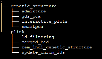
The results are stored in the folder ./genetic_structure and inside we have subfolders of each PCA, Admixture and interactiv plots. In subfolder /plink are stored files after modifying and filtering steps.
folders
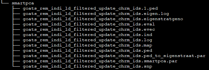
Each PCA has its own folder with eigenvectors and eigenvalues: 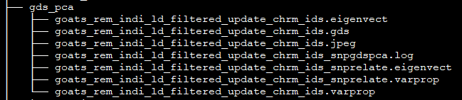
folders
Folder admixture contains Q-matrices for each K value together with interactive plot of optimal K:

folders
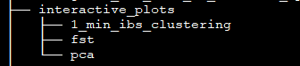
Interactive plots of PCA and both NJ trees are stored here:
folders
Let’s take a look at the PCA plots first. On both of them our samples cluster into three groups. In the first one we can found all breeds of domestic goats from Switzerland. In another cluster are Alpine ibexes and in the third one are Bezoar wild goats.

image description
Figure 1: Interactive plots of both Principal Component Analyses
Program Admixture estimated the optimal number of clusters at five. As we can see on Figure 2, four Swiss goats (Booted, Chamois colored, Peacock and Saanen) are showing very similar genomic structures. Appenzell and Toggenburg goat breeds have distinct and more homogeneous structures with some individual goats that share segments with other breeds from Switzerland. Both wild species, Alpine ibex and Bezoar, have uniform genetic structures.
 Figure 2: Population structures of our dataset
The NJ tree of IBS-based (Figure 3) distances positioned the branches of Swiss goats according to their breeds. Alpine ibexes and Bezoar wild goats formed their own clade, inside of which we can see clear distinction between the two species. According to that distribution was also the layout of Fst-based NJ tree (Figure 4), but, unlike the IBS-based tree, here we have population’ divergence.
 Figure 3: A neighbor-joining tree constructed with
matrix of IBS distances between individuals
Figure 3: A neighbor-joining tree constructed with
matrix of IBS distances between individuals
 Figure 4: A neighbor-joining tree constructed with Fst
distances between populations
Figure 4: A neighbor-joining tree constructed with Fst
distances between populations
5. Generating the interactive plots without running the workflow
For generating the interactive pca plot only (withut re-running the workflow), one can use the following command:
python3 plot_interactive_pca.py <eigenvect_file> <eigenval_file> pop_markershape_col.txt pca.yml <output_prefix>
The python script is located in the bin folder of scalepopgen. **** and **** are located in the respective output folders of smartpca and gds_pca. The yaml file is located in “/parameters/plots/” folder. pop_markershape_col.txt is located in the folder of “interactive_plots/pca/” or one can also create this tab-delimited file with this format: the first column is pop_id, the second column is shape_id, the third column is hex color code. Refer to “./extra/markershapes.txt” to see the list of shapes implemented in this bokeh-dependent python script. The parameters of the yaml files are described below:
plot_width: plot-width size in pixel
plot_height: plot-height size in pixel
pc_x_to_plot: which pc to plot on the x-axis
pc_y_to_plot: which pc to plot on the y-axis
fill_alpha: fill-color intensity
line_alpha: line-color intensity
marker_size : size of the markers to be plotted; input should be boolean; True or False
show_sample_label: whether or not to show the sample label for each dot during hovering.
For plotting the large number of samples and population, increase the plot_width and plot_height size, reduce the marker_size and set show_sample_label to false
Next, the admixture plot can be also generated with the following command:
python3 plot_interactive_q_mat.py -q <Q_matrix_file> -f <plink_fam_file> -y admixture.yml -c color.txt -o <output_prefix> -s plot_pop_order.txt
The python script located in the bin folder of scalepopgen. **** is located in the respective output folder of admixture. The file is located in folder **./plink/update_chrom_ids/.fam*. Text files**color.txtandplot_pop_order.txtcan be created by the user. Filecolor.txt** has hex color codes listed in one column:
#FF0000
#00FF00
#0000FF
#FFFF00
#FF00FF
#00FFFF
#FFA500
#800080
#008000
#800000
Similarly, in file plot_pop_order.txt population IDs are listed in one column according to the order they should be plotted:
Appenzell
Booted
ChamoisColored
Peacock
Saanen
Toggenburg
Bezoar
AlpineIbex
The yaml file admixture.yml is located in “/parameters/plots/” and it cointains parameters described below:
width: plot-width size in pixel
height: plot-height size in pixel
bar_width: the width of each sample bar
sample_label_orientation: degrees of anlge at which the sample labels should be written
pop_label_orientation: degrees of anlge at which the population labels should be written
space_pop_group: the width of space between populations
legend_font_size: font size of the legend
num_legend_per_col: number of different K per column
label_font_size: font size of the labels
fil_alpha: fill-color intensity
For generating the IBS-dist interactive NJ trees, one can use the following command:
python3 make_ibs_dist_nj_tree.py -r <outgroup> -i <square_mat_mdist_file> -m <mdist.id_file> -c pop_sc_color.map -y ibs_nj.yml -o <output_prefix>
The python script is located in the bin folder of scalepopgen. **** refers to the population to be used for rooting the tree, **** refers to the sqaure matrix of 1-ibs distance between pairwise samples and generated by plink1.9, <mdist.id_file> refers to id file generated along with the square matrix by plink1.9, pop_sc_color.map* is the tab-delimited file containing the first column as pop_id, second column as sample size and the third column as hex color code. Also generated by the workflow and saved in the output folder aspop_sc_color.map**. The yml file is located in “parameter/plots/” folder. The parameter of the yml files are described below:
width: plot-width size in pixel
height: plot-height size in pixel
layout: the tree layout, valid options: 'c','r','d', for circular, right and down layout of the tree
tip_label_align: whether or not to align the tip labels; input should be boolean; True or False
tip_label_font_size: the font size of the tip labels, default: "12px"
edge_widths: the width of edges, default: 1
node_sizes: the size of nodes, default:6
node_hover: whether or not to show details info of the node while hovering; input should be boolean; True or False
The python script can also be run directly using the file containing tree in newick format. For more details run “python3 make_ibs_dist_nj_tree.py -h”. As the python script is dependent on Toytree, for more details of these parameters, refer to Toytree documentation.
For generating the fst-based NJ tree, one can use the following command:
python3 make_fst_dist_nj_tree.py -i <fst_summary_file_generated_by_plink2> -r <outgroup> -o <output_prefix> -y fst_nj.yml -c pop_sc_color.map
References
Please cite the following papers if you use this sub-workflow in your study:
[1] Alexander, D. H., Novembre, J., & Lange, K. (2009). Fast model-based estimation of ancestry in unrelated individuals. Genome research, 19(9), 1655-1664. https://doi.org/10.1101/gr.094052.109
[2] Patterson, N., Price, A. L., & Reich, D. (2006). Population structure and eigenanalysis. PLoS genetics, 2(12), e190. https://doi.org/10.1371/journal.pgen.0020190
[3] Price, A. L., Patterson, N. J., Plenge, R. M., Weinblatt, M. E., Shadick, N. A., & Reich, D. (2006). Principal components analysis corrects for stratification in genome-wide association studies. Nature genetics, 38(8), 904-909. https://doi.org/10.1038/ng1847
[4] Zheng, X., Levine, D., Shen, J., Gogarten, S. M., Laurie, C., & Weir, B. S. (2012). A high-performance computing toolset for relatedness and principal component analysis of SNP data. Bioinformatics (Oxford, England), 28(24), 3326-3328. https://doi.org/10.1093/bioinformatics/bts606
[5] Francis, R. M. (2017). pophelper: an R package and web app to analyse and visualize population structure. Mol Ecol Resour, 17: 27–32. doi:10.1111/1755-0998.12509
[6] Huerta-Cepas, J. et al.,(2016). ETE 3: Reconstruction, Analysis, and Visualization of Phylogenomic Data, Molecular Biology and Evolution, Volume 33, Issue 6, June 2016, Pages 1635–1638, https://doi.org/10.1093/molbev/msw046.
[7] Eaton, Deren. (2019). Toytree: A minimalist tree visualization and manipulation library for Python. Methods in Ecology and Evolution. 11. 10.1111/2041-210X.13313.
[8] Di Tommaso, P., Chatzou, M., Floden, E. et al. Nextflow enables reproducible computational workflows. Nat Biotechnol 35, 316-319 (2017). https://doi.org/10.1038/nbt.3820
License
MIT